Annual maps

How to make some quick maps with the ARCOS api.

First, let’s load some packages.

# Uncomment and run the lines below to see if you have the packages required already installed
# packages <- c("dplyr", "ggplot2", "jsonlite", "knitr", "geofacet", "scales")
# if (length(setdiff(packages, rownames(installed.packages()))) > 0) {
#   install.packages(setdiff(packages, rownames(installed.packages())), repos = "http://cran.us.r-project.org") # }

# These are all the packages you'll need to run everything below 

library(dplyr)
library(ggplot2)
library(arcos)
library(jsonlite)
library(knitr)
library(geofacet)
library(scales)

states <- combined_buyer_annual(key="WaPo")

kable(head(states))

BUYER_DEA_NO	BUYER_BUS_ACT	BUYER_COUNTY	BUYER_STATE	year	DOSAGE_UNIT
A90777889	RETAIL PHARMACY	KINGS	NY	2006	110700
A90777889	RETAIL PHARMACY	KINGS	NY	2007	119100
A90777889	RETAIL PHARMACY	KINGS	NY	2008	100300
A90777889	RETAIL PHARMACY	KINGS	NY	2009	92630
A90777889	RETAIL PHARMACY	KINGS	NY	2010	65860
A90777889	RETAIL PHARMACY	KINGS	NY	2011	72030

We’ve pulled every pharmacy across the country and how many pills they sold per year.

Let’s aggregate and combine by states and year.

annual_states <- states %>% 
  group_by(BUYER_STATE, year) %>% 
  summarize(pills=sum(DOSAGE_UNIT)) %>% 
  filter(!is.na(BUYER_STATE))
#> `summarise()` has grouped output by 'BUYER_STATE'. You can override using the
#> `.groups` argument.

kable(head(annual_states))

BUYER_STATE	year	pills
AE	2006	330
AK	2006	15667010
AK	2007	17272433
AK	2008	18707811
AK	2009	20160949
AK	2010	21012703

Looks good. Let’s use the geofacet package to map out the annual pill trends.

ggplot(annual_states, aes(year, pills)) +
  geom_col() +
  facet_geo(~ BUYER_STATE, grid = "us_state_grid2") +
    scale_x_continuous(labels = function(x) paste0("'", substr(x, 3, 4))) +
  scale_y_continuous(label=comma) +
  labs(title = "Annual oxycodone and hydrocodone pills by state",
    caption = "Source: The Washington Post, ARCOS",
    x = "",
    y = "Dosage units") +
  theme(strip.text.x = element_text(size = 6))

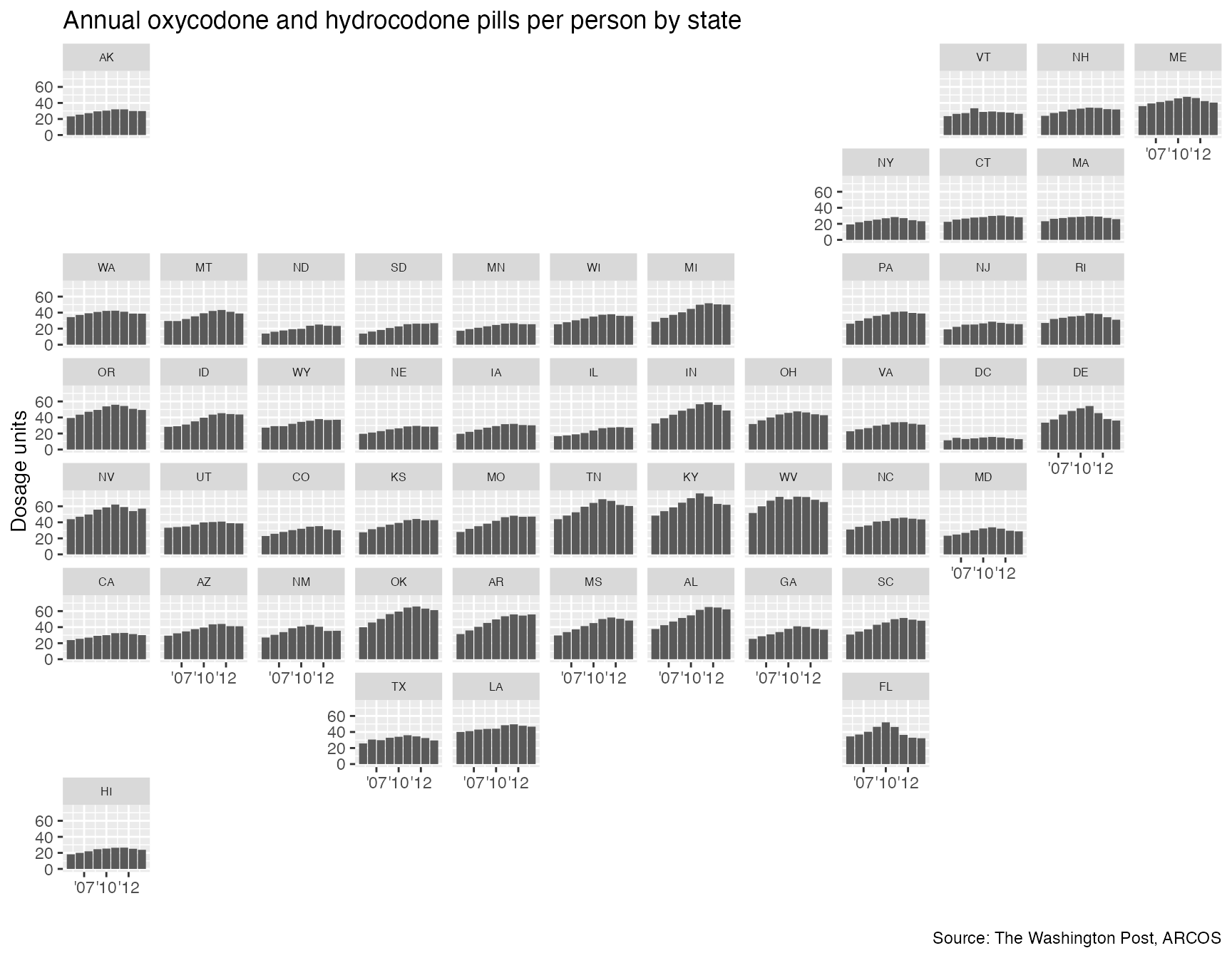
This is nice but Florida, California, and Texas stand out because of their higher population.

We should normalize this with population.

Get the annual state population with state_population().

population <- state_population(key="WaPo")

kable(head(population))

BUYER_STATE	year	population
AL	2009	4633360
AK	2009	683142
AZ	2009	6324865
AR	2009	2838143
CA	2009	36308527
CO	2009	4843211

Now, we join the two data sets.

Adjust for population.

annual_states_joined <- left_join(annual_states, population) %>% 
  filter(!is.na(population))
#> Joining with `by = join_by(BUYER_STATE, year)`

kable(head(annual_states_joined))

BUYER_STATE	year	pills	population
AK	2006	15667010	675302
AK	2007	17272433	680300
AK	2008	18707811	687455
AK	2009	20160949	683142
AK	2010	21012703	691189
AK	2011	22444775	700703

Do some math…

annual_states_joined <- annual_states_joined %>% 
  mutate(pills_per=pills/population)

kable(head(annual_states_joined))

BUYER_STATE	year	pills	population	pills_per
AK	2006	15667010	675302	23.20001
AK	2007	17272433	680300	25.38944
AK	2008	18707811	687455	27.21314
AK	2009	20160949	683142	29.51209
AK	2010	21012703	691189	30.40081
AK	2011	22444775	700703	32.03180

Map it out again this time per capita.

ggplot(annual_states_joined, aes(year, pills_per)) +
  geom_col() +
  facet_geo(~ BUYER_STATE, grid = "us_state_grid2") +
    scale_x_continuous(labels = function(x) paste0("'", substr(x, 3, 4))) +
  scale_y_continuous(label=comma) +
  labs(title = "Annual oxycodone and hydrocodone pills per person by state",
    caption = "Source: The Washington Post, ARCOS",
    x = "",
    y = "Dosage units") +
  theme(strip.text.x = element_text(size = 6))